Planar Stress and Planar Deformation
A wide variety of structures within the field of civil engineering can
be formulated as two-dimensional elasticity problems. These structures
have the appearance of right prisms.
Planar state of stress:
If one dimension of such a structure (thickness = t) is much less than
the other two which form a plane, and loads are applied only to this
plane, we say it is a planar stress problem.
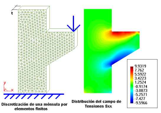
Examples of structures involving planar stress are wide-edged beams,
plates with loads tangential to their plane, and buttress dams.
Structures with planar deformation
It is said that a structure has planar deformation if, having one
dimension (length) much greater than the other two, it is under loads
evenly distributed only along this length and within planes orthogonal
to the line that joins the centers of gravity of the various cross
sections.
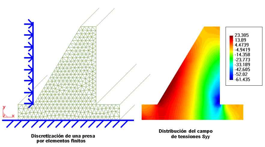
Among this type of structure are gravity dams, pipes with interior
pressure, and retaining walls.
Defining the geometry:
Since this is a two-dimensional problem, the geometry must be defined
on the plane Z=0.
The figure shows the geometry of a gravity dam composed of a series
of line segments between two points. These segments form three
surfaces.
This geometry must be defined along the X and Y local axes, with Z=0.
It is very important, in order to avoid confusion when assigning
boundary conditions, to understand the way in which the local axes
are assigned relative to the different entities and relative to the
global axes.
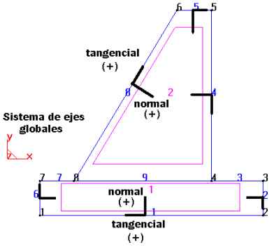
The following figure shows how the global axes are the ones GiD
proposes when defining the geometry.
Concerning the local axes, it is necessary to define only the axis
on the lines, as these lines are the ones forming the surfaces to
which loads or constraints will be applied. This way, the normal
positive axis of any line is defined as that which is directed
normally to the line and towards the interior of the surface that
the line defines.
On each surface, the tangential axis is defined in the direction of
the line and counterclockwise, as illustrated in the following figure.
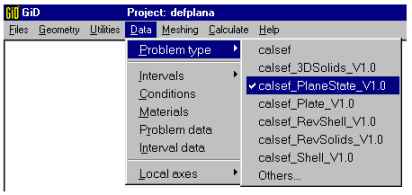
Once the geometry is defined, the problem type to solve may be
specified. Since our example is a Planar State problem, select the
module Calsef_PlaneState_V1.0
Boundary conditions ("Conditions"):
For this kind of problem (Planar State) Calsef offers the following
boundary conditions:
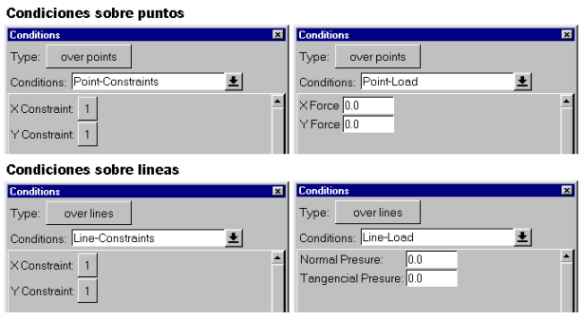
The axes on which these conditions are specified are the global axes,
except in the case of Line-Load, when the loads are Normal_Pressure and
Tangential_Pressure. This means that these loads are applied along the
directions of the local axes for each line, Normal_Pressure being the
direction normal to the line and positive inward on the surface.
As to the tangential load, Tangential_Pressure, its direction is that
of the line, positive and clockwise in respect to the surface.
The loads applied to a line are per unit of length of that line.
The following figure shows a series of constraints applied to the
geometry defined in the previous step. These constraints may be
represented graphically using GiD's graphics tools.

Defining the materials ("Materials")
Materials must be assigned to the surfaces forming the geometry.
For our example, select concrete as the material for the dam and
generate a new material for the floor.

The final configuration of these two selected materials may be viewed
using GiD's graphics tools.
Specific data of the problem ("Problem Data")
The example being solved is one of planar deformation. However, by
default Calsef is ready for a planar stress problem. Therefore, the
problem type must be changed.
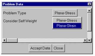
First, make the change in the "Problem Type" box and then make sure to
click on "Accept Data" in order to save the changes made.
In this window there are other options such as whether or not to
include self-weight in the analysis. Make sure the weight is always
oriented along the Y axis and toward the negative values.
Generating the mesh ("Meshing"):
The example must be solved with a mesh of quadratic triangular
elements. Following are the steps for generating the mesh.
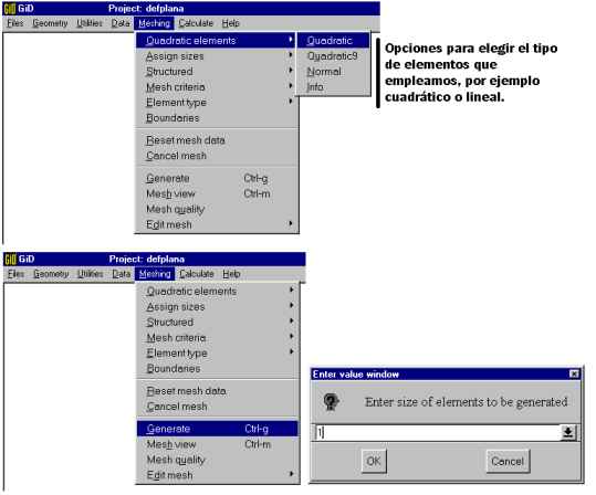
In this case, the size of the finite elements is 1, in accord with
the dimensions of the dam. The resulting mesh is the following:

Now the project is ready to be saved ("Save") and calculated.
Finite elements available:
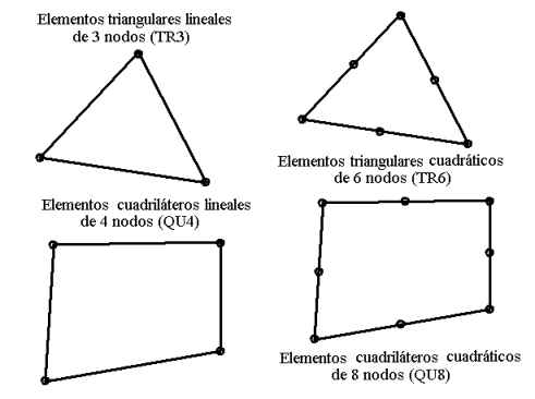
Remember that the generation of meshes must always be based on
elements available in Calsef. Otherwise, the information will not
be properly understood and the problem will not be solved.
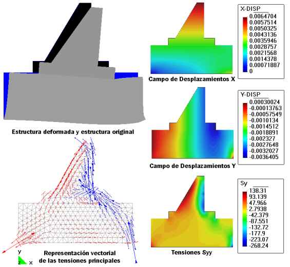
Results:
Once the structure in question has been solved, the results may be
visualized in different ways.
This type of planar problem generates the following results:
· Deformation along a global X axis (X-Def)
· Deformation along a global Y axis (Y-Def)
These deformations are described relative to the global axes of the
problem both in direction as well as positive values. If the data are
entered in the SI, the results will be in meters.
· Stress along the global X axis (Sx)
· Stress along the global Y axis (Sy)
· Stresses tangential to the XY plane (Sxy)
These stresses are described in relation to the global axes of the
problem. Their sign is positive for tension and negative for
compression. If the data are entered in the SI, the results (stress)
will be in N/m2.
· Principal stresses (Si, Sii)
The principal stresses are studied with reference to the principal
axes. These axes may be visualized using GiD's graphics tools.
The sign of these stresses will be positive for tension and negative
for compression.
Go back