Using GiD
This chapter illustrates the use of GiD for describing the characteristics that will ultimately define our model. The following steps are valid for all the problem types available in Calsef. The steps are ordered in a logical sequence so that the user may follow them from the beginning to the end of the problem-solving process. Although some of the steps (sub-processes) may be applied at different stages of the overall process, we suggest the sequence described in this chapter as it guards against omitting any steps.

Defining the geometry:

The geometry may be defined using GiD's graphics tools, described in detail in The GiD User's Manual. Remember: 1) planar problems such as planar states, solids of revolution, and plates involve meshes over planar surfaces (Z=0 plane); 2) shells involve meshes over surfaces in space; and 3) 3D solids involve meshes over volumes.
Volumes are generated based on the surfaces limiting them; surfaces, based on the lines; and lines, based on the points.

To generate the mesh properly, it is essential to avoid duplicating any of the basic geometric entities.
Visualizing the labels that correspond to all the entities will ensure that one entity is not superimposed over another.

It is also important to keep in mind the axes used and their (positive) directions so as to correctly orient the loads and interpret the results for each problem type.
These sign conventions vary according to the theory applied in each case. These aspects of analysis follow the theories described in the book, Cálculo de Estructuras por el Método de los Elementos Finitos by Eugenio Oñate. Nevertheless, the present manual describes the axes used in each problem type.
Also keep in mind that each problem type requires that the structure be oriented in a certain way. For example, in a problem with rotational symmetry, the axis is taken as the Y axis. Therefore, the geometry must be defined in the quadrant with X>0. Moreover, since it is a planar problem, the geometry must be situated on the plane Z=0. Further on in this manual, these aspects are explained in greater detail for each problem type

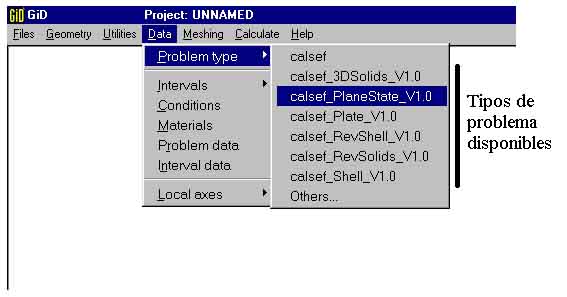
Selecting the problem type ("Problem type"):

Once the geometry is defined, the problem type to solve must be selected according to the menu shown:



On selecting the problem type, assign the boundary conditions, loads, materials, and data for the particular structure type in question.
Now we are ready to begin the definitions of our model problem.

Adopting a unit system:

It is essential to adopt a coherent system of units in order to define a geometry as well as to enter materials characteristics and load values.
To ensure coherence, we recommend using the international system (SI). In other words, length should be expressed in meters, and forces should be expressed in newtons. Accordingly, deformation results will be in meters, gyration results will be in radians, and forces will be in newtons. The rest of the units will be a combination of these three (e.g., bending moments in N/m).

Assigning boundary conditions ("Conditions"):

Each problem type has its own boundary conditions and loads, but the way of assigning them is common to all problem types.
Loads and boundary conditions may be assigned either to the geometry or to the mesh of the problem. The difference between both procedures is that if we assign the conditions to the geometry, every time a different mesh is generated based on this geometry, the conditions will be translated to each mesh. In contrast, if the conditions are applied to the mesh directly, this information will be lost when the mesh is modified.
We suggest applying the boundary conditions to the geometry and NOT to the mesh. This procedure guards against omitting a condition when a new mesh is generated. Furthermore, it enables the user to sort complicated situations such as applying loads to lines of elements. If the conditions have been applied to the geometry, it will be clear whether or not a specific element is in the line receiving the load.
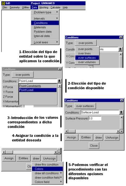
Before applying conditions to entities, first select which entity will receive the conditions: points, lines, surfaces, or volumes.
Then select the type of conditions to apply as shown on the menu.
The menu asks for the corresponding values of the selected boundary condition(s). In the case of restrictions of movement, 1 indicates restriction in the degrees of freedom, while 0 indicates no restriction in the degrees of freedom.
Now assign the previously defined conditions to the entities in question.
GiD is equipped with various tools for visualizing the conditions applied.
Use of these tools is recommended for avoiding errors in procedure.




Careful attention must be paid to the axes to which these conditions are applied. The axes might be for certain conditions within global coordinates and for other conditions in local coordinates of the entity. In general, pressures (distributed loads) applied on lines or surfaces use local coordinates, while forces (concentrated loads) applied on nodes use global coordinates. This subject, as well as the definition of axes for each entity, is explained in greater detail for the different loads in each problem type.

Assigning and defining the materials ("Materials"):

Depending on the problem type, the characteristics to be entered will be different. But the methodology used for assigning the materials is always the same.



The program already has two materials previously defined by default. However, any material may be defined simply by entering a name in the "New Material" box and then modifying the corresponding values.
IMPORTANT. After modifying the value of a material or entering a new material, ALWAYS click on "Accept Data" in order to save the changes made. This procedure is explained in greater detail in the GiD User's Manual.
For coherence, values must all be in the same units.
Once a material is selected or entered, it must be assigned to the corresponding entities.
The material must be assigned to the proper entity type under study. For example, a 3D problem will be defined by a volume in space.
Therefore, a material must be assigned to the volume - not to the surfaces or lines defining the volume.
In other words, a material is assigned to an entity so that when the mesh is generated for the entity, the characteristics of the assigned material will pass automatically to the elements that form the mesh. Therefore, if the mesh is composed of 3D solid elements, given that it is a problem of spatial volume, the material must be assigned to the entities of volume.
All the entities defining the mesh of the model must have a material assigned to them. GiD is equipped with a visualization system which enables the user to color one or all of the materials present in the model in order to verify that all the entities defining the model have been assigned a material. Just as in the case of the boundary conditions, using these verification tools is highly recommended in order to avoid errors.



Specific data of the problem ("Problem data"):

At this stage of the process, the specific data of the problem must be defined, i.e., whether weight is to be considered, or whether it is a planar problem or stress or of deformation.



The program will show the different options available for each individual case. Remember to click on the "Accept Data" box whenever the values of the problem are modified.

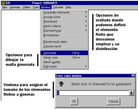
Generating the finite-element mesh ("Meshing") :

GiD is equipped with a mesh generator that offers a broad range of possibilities.
The most significant options are generating meshes with linear or with quadratic finite elements, depending on whether or not the problem type in question permits these options. The mesh may be structured according to the type of surface or volume adopted. It may also be made denser in zones requiring greater precision.
These tools are explained in greater detail in the GiD User's Manual.
However, a default mesh may also be generated without having selected any of the previous options, by directly clicking on "Generate." This will define a mesh with the simplest elements available for each problem type. For example, in the case of a planar structure, triangular elements of three nodes are generated. In the case of three-dimensional solids, tetrahedral elements of four nodes are generated.
Before generating a mesh, the average size of the elements must be decided. Make sure that the sizes entered are not too small for the program to later solve numerically. Although for each type of problem there is a range of possibilities for finite elements, remember that Calsef must be able to solve the mesh generated.
GiD will generate the mesh over the highest rank entity. In other words, if we define a volume with surfaces that are, in turn, defined by lines, what we want is the mesh over the volume. This is what GiD understands. Clicking on "Generate" will define the mesh over the volume with finite elements of volume.
Care must be taken not to generate meshes for two different entity levels in the same problem. If we are working with volumes, all the surfaces must be used to define volumes. Accordingly, when the mesh is generated, only volume elements will be present.
As a safety measure, in the present version of Calsef, if the user indicates that the problem involves three-dimensional volumes but defines some elements as planar or two-dimensional, an error-warning box will come up.



When a mesh is generated. GiD takes the previously fixed boundary conditions and materials characteristics for each entity and assigns them to each element or node generated. Therefore, any modification in these data means repeating the meshing process.
The mesh menu includes the option "Mesh View," which enables the user to visualize the mesh generated. This option is very important for verification of the mesh, which will ultimately determine the real geometry to calculate.

Saving a project and calculating:

The last step in defining a project is "Save as." This is the option to select in the case of a new project that is to be written onto a disk. If it is a modified preexisting project, this step will be simply "Save."
The exact way in which GiD saves files is explained in the bibliography previously mentioned.
Once the problem is saved, the user may begin calculating it.
Click on "Calculate." This will automatically send all the information entered in GiD to Calsef, which will solve the problem numerically.



Visualizing the results ("Postprocess"):

After the problem is calculated and GiD says the calculation is finished, the user may change to the "postprocess" mode in order to visualize the results.
The results will be rendered in different forms depending on the type of problem.
The form of the results is dealt with further on in this manual in the chapters on problem types. In general, though, the results usually involve deformation and sheering or tensile stresses.



In the postprocess, the results may be visualized in different ways. Therefore, to fully benefit from the postprocess possibilities, we recommend reading the corresponding chapters in the GiD User's Manual.

Go back

---